What this benchmark measures
This vignette evaluates how well different context-retrieval strategies help an LLM answer R coding tasks. The benchmark asks:
Given a natural-language task description and an R project, which retrieval strategy gives an LLM the context it needs to produce correct, runnable R code?
Each strategy is judged by how often the LLM response:
-
Parses as valid R syntax
(
syntax_valid) -
Runs without error when
eval(parse(...))is called (runs_without_error) -
Mentions the right functions – the fraction of
ground-truth node names found in the generated code
(
nodes_score)
These three components are combined into a single composite score between 0 and 1:
score = 0.25 * syntax_valid
      + 0.45 * nodes_score
      + 0.30 * runs_without_error
A score of 1.0 means the response parsed, ran, and referenced every expected function/object. A score of 0 means it failed on all three.
Retrieval strategies compared
| Strategy | How context is retrieved | Token cost |
|---|---|---|
graph_rag_tfidf |
Graph-RAG: graph traversal with TF-IDF similarity to query | Low – only relevant nodes |
graph_rag_tfidf_noseed |
Graph-RAG: TF-IDF traversal seeded by the query itself, no caller-specified seed node | Low |
graph_rag_ollama |
Graph-RAG: graph traversal with Ollama vector similarity | Low – only relevant nodes |
graph_rag_mcp |
Graph-RAG: traversal via the rrlmgraph-mcp MCP server (requires running server) | Low |
graph_rag_agentic |
RLM-Graph: LLM drives MCP tool calls (find_callers,
find_callees, search_nodes,
get_node_info) iteratively |
Low – LLM-selected nodes only |
full_files |
Every source file in the project dumped verbatim (upper baseline) | Very high |
bm25_retrieval |
Files ranked by BM25 score against the task description (no graph) | Medium |
term_overlap |
Files ranked by word overlap with the task description (no graph) | Medium |
no_context |
No code context sent – LLM must answer from training data alone (lower baseline) | Zero |
random_k |
Five randomly sampled code chunks (random baseline) | Low |
The two baselines to beat are:
-
no_context– if a strategy cannot beat this, it is useless. -
full_files– if a strategy beats this at lower token cost, graph retrieval is providing genuine value.
Results are loaded from
inst/results/benchmark_results.rds. They are regenerated
automatically four times daily (03:00, 09:00, 15:00, and 21:00 UTC, and
on demand) by the run-benchmark CI workflow using GitHub
Models (gpt-4o-mini).
Results
results_path <- system.file(
  "results", "benchmark_results.rds",
  package = "rrlmgraphbench"
)
results_available <- file.exists(results_path)
if (!results_available) {
  message(
    "benchmark_results.rds not found.\n",
    "Trigger the run-benchmark GitHub Actions workflow to generate results,\n",
    "or run run_full_benchmark() locally with .dry_run = TRUE for a quick test."
  )
} else {
  all_results <- readRDS(results_path)
  # Drop rows where the LLM call failed (e.g. rate-limit exhaustion at end of
  # daily quota). These NA scores would propagate through statistics and plots.
  n_na <- sum(is.na(all_results$score))
  if (n_na > 0L) {
    message(n_na, " row(s) with NA score dropped (rate-limit failures).")
    all_results <- all_results[!is.na(all_results$score), ]
  }
  knitr::kable(
    head(all_results[, c(
      "task_id", "strategy", "trial", "score",
      "syntax_valid", "runs_without_error", "total_tokens"
    )], 6),
    caption = paste0(
      "First 6 rows of raw results. 'score' is the composite 0-1 metric. ",
      "'syntax_valid' and 'runs_without_error' are 0/1 indicators. ",
      "'total_tokens' is the sum of input + output tokens billed."
    )
  )
}| task_id | strategy | trial | score | syntax_valid | runs_without_error | total_tokens |
|---|---|---|---|---|---|---|
| task_049_hard_bd_shiny | graph_rag_tfidf | 1 | 1.00 | TRUE | TRUE | 539 |
| task_049_hard_bd_shiny | graph_rag_tfidf | 2 | 1.00 | TRUE | TRUE | 539 |
| task_049_hard_bd_shiny | graph_rag_tfidf | 3 | 1.00 | TRUE | TRUE | 544 |
| task_049_hard_bd_shiny | graph_rag_tfidf | 4 | 1.00 | TRUE | TRUE | 539 |
| task_049_hard_bd_shiny | graph_rag_tfidf | 5 | 1.00 | TRUE | TRUE | 549 |
| task_049_hard_bd_shiny | graph_rag_tfidf_noseed | 1 | 0.91 | TRUE | TRUE | 531 |
Summary statistics
Each metric below is averaged across all tasks and trials for a given strategy.
| Column | Meaning |
|---|---|
n |
Total trials (tasks x trials per task) |
mean_score |
Average composite score (0-1); higher is better |
sd_score |
Standard deviation of per-trial scores |
ci_lo_95 / ci_hi_95
|
95% confidence interval for the mean score |
mean_total_tokens |
Average tokens consumed per trial (input + output) |
hallucination_rate |
Fraction of trials where at least one invented function/argument was detected |
if (results_available) {
  stats <- compute_benchmark_statistics(all_results)
  knitr::kable(
    stats$summary[, c(
      "strategy", "n", "mean_score", "sd_score",
      "ci_lo_95", "ci_hi_95", "mean_total_tokens", "hallucination_rate"
    )],
    digits = 3,
    caption = "Summary: mean score, 95% CI, token usage, and hallucination rate per strategy."
  )
}| strategy | n | mean_score | sd_score | ci_lo_95 | ci_hi_95 | mean_total_tokens | hallucination_rate |
|---|---|---|---|---|---|---|---|
| graph_rag_tfidf | 40 | 0.859 | 0.135 | 0.816 | 0.902 | 705.550 | 0.725 |
| graph_rag_tfidf_noseed | 40 | 0.834 | 0.170 | 0.779 | 0.888 | 643.200 | 0.625 |
| graph_rag_ollama | 40 | 0.862 | 0.151 | 0.814 | 0.910 | 733.450 | 0.750 |
| full_files | 40 | 0.869 | 0.104 | 0.836 | 0.902 | 1589.200 | 0.750 |
| term_overlap | 40 | 0.855 | 0.122 | 0.816 | 0.894 | 1579.175 | 0.750 |
| bm25_retrieval | 36 | 0.850 | 0.101 | 0.816 | 0.884 | 1001.389 | 0.722 |
| no_context | 35 | 0.821 | 0.149 | 0.769 | 0.872 | 304.571 | 0.571 |
| graph_rag_mcp | 35 | 0.836 | 0.106 | 0.799 | 0.872 | 675.971 | 0.714 |
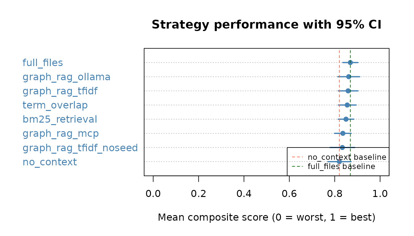
Score distribution (with confidence intervals)
The dot chart below shows each strategy’s mean score. Horizontal bars are 95% confidence intervals. Strategies are sorted best-to-worst. A strategy is significantly better than another only if the confidence intervals do not overlap.
if (results_available) {
  summary_df <- stats$summary
  summary_df <- summary_df[order(summary_df$mean_score, decreasing = FALSE), ]
  n_s <- nrow(summary_df)
  dotchart(
    summary_df$mean_score,
    labels = summary_df$strategy,
    xlab   = "Mean composite score (0 = worst, 1 = best)",
    main   = "Strategy performance with 95% CI",
    pch    = 19,
    col    = "steelblue",
    xlim   = c(0, 1)
  )
  segments(
    x0  = summary_df$ci_lo_95,
    x1  = summary_df$ci_hi_95,
    y0  = seq_len(n_s),
    lwd = 2,
    col = "steelblue"
  )
  abline(
    v = summary_df$mean_score[summary_df$strategy == "no_context"],
    lty = 2, col = "tomato", lwd = 1
  )
  abline(
    v = summary_df$mean_score[summary_df$strategy == "full_files"],
    lty = 2, col = "darkgreen", lwd = 1
  )
  legend("bottomright",
    legend = c("no_context baseline", "full_files baseline"),
    col = c("tomato", "darkgreen"),
    lty = 2, lwd = 1, cex = 0.8
  )
}
Token Efficiency Ratio (TER)
TER = (strategy mean score / strategy mean tokens) / (full_files mean score / full_files mean tokens).
A TER > 1 means the strategy delivers more
score per token than dumping the entire project. This is the key
metric for assessing whether graph-based retrieval is worth deploying in
production over the brute-force full_files approach.
if (results_available) {
  ter_df <- data.frame(
    strategy = names(stats$ter),
    TER = round(stats$ter, 3),
    interpretation = ifelse(
      is.na(stats$ter), "N/A (baseline)",
      ifelse(stats$ter > 1,
        "More efficient than full_files",
        "Less efficient than full_files"
      )
    )
  )
  ter_df <- ter_df[order(ter_df$TER, decreasing = TRUE, na.last = TRUE), ]
  knitr::kable(ter_df,
    row.names = FALSE,
    caption = paste0(
      "Token Efficiency Ratio (TER) vs full_files baseline. ",
      "TER > 1: strategy achieves higher score-per-token than full_files. ",
      "TER < 1: strategy is less efficient."
    )
  )
}| strategy | TER | interpretation |
|---|---|---|
| no_context | 4.927 | More efficient than full_files |
| graph_rag_tfidf_noseed | 2.371 | More efficient than full_files |
| graph_rag_mcp | 2.262 | More efficient than full_files |
| graph_rag_tfidf | 2.227 | More efficient than full_files |
| graph_rag_ollama | 2.149 | More efficient than full_files |
| bm25_retrieval | 1.552 | More efficient than full_files |
| term_overlap | 0.990 | Less efficient than full_files |
| full_files | NA | N/A (baseline) |
Hallucination analysis
A hallucination is any invented function name, invalid argument, or wrong package namespace in the LLM response. Hallucinations make generated code fail silently or with confusing errors.
if (results_available) {
  hall_df <- stats$summary[, c("strategy", "hallucination_rate")]
  hall_df$hallucination_rate <- round(hall_df$hallucination_rate, 3)
  hall_df <- hall_df[order(hall_df$hallucination_rate), ]
  hall_df$verdict <- ifelse(
    hall_df$hallucination_rate == 0, "None detected",
    ifelse(hall_df$hallucination_rate < 0.1, "Low (< 10%)",
      ifelse(hall_df$hallucination_rate < 0.25, "Moderate (10-25%)", "High (> 25%)")
    )
  )
  knitr::kable(hall_df,
    row.names = FALSE,
    caption = paste0(
      "Hallucination rate per strategy. ",
      "Defined as: fraction of trials with >= 1 invented function, ",
      "invalid argument, or wrong namespace."
    )
  )
}| strategy | hallucination_rate | verdict |
|---|---|---|
| no_context | 0.571 | High (> 25%) |
| graph_rag_tfidf_noseed | 0.625 | High (> 25%) |
| graph_rag_mcp | 0.714 | High (> 25%) |
| bm25_retrieval | 0.722 | High (> 25%) |
| graph_rag_tfidf | 0.725 | High (> 25%) |
| graph_rag_ollama | 0.750 | High (> 25%) |
| full_files | 0.750 | High (> 25%) |
| term_overlap | 0.750 | High (> 25%) |
Hallucination type breakdown (where available):
if (results_available && "hallucination_details" %in% names(all_results)) {
  # Use keepNA = FALSE so NA entries in hallucination_details are excluded,
  # preventing NA propagation into strsplit / regmatches / barplot names.arg.
  non_empty <- !is.na(all_results$hallucination_details) &
    nzchar(all_results$hallucination_details)
  details_flat <- unlist(strsplit(all_results$hallucination_details[non_empty], "; "))
  details_flat <- details_flat[!is.na(details_flat) & nzchar(details_flat)]
  if (length(details_flat) > 0) {
    known_types <- c("invented_function", "invalid_argument", "wrong_namespace")
    type_pattern <- regmatches(
      details_flat,
      regexpr(paste(known_types, collapse = "|"), details_flat)
    )
    type_counts <- sort(table(type_pattern), decreasing = TRUE)
    # Only plot understood types; skip any unknown category gracefully.
    keep <- names(type_counts) %in% known_types
    type_counts <- type_counts[keep]
    if (length(type_counts) > 0L) {
      label_map <- c(
        invented_function = "Invented\nfunction\n(e.g. foo::bar\nthat doesn't exist)",
        invalid_argument  = "Invalid\nargument\n(e.g. wrong\nparam name)",
        wrong_namespace   = "Wrong\nnamespace\n(e.g. pkg1::fn\ninstead of pkg2::fn)"
      )
      barplot(
        type_counts,
        main = "Hallucination types across all strategies",
        ylab = "Count of occurrences",
        xlab = "Type",
        col = c("tomato", "goldenrod", "steelblue")[seq_along(type_counts)],
        names.arg = label_map[names(type_counts)]
      )
    } else {
      message("No known hallucination types detected in the loaded results.")
    }
  } else {
    message("No hallucinations detected in the loaded results.")
  }
}
#> No known hallucination types detected in the loaded results.
Pairwise statistical tests
Each pair of strategies is compared using a Welch t-test (robust to unequal variance). P-values are Bonferroni-corrected for multiple comparisons. Cohen’s d measures practical effect size: |d| < 0.2 = negligible, 0.2-0.5 = small, 0.5-0.8 = medium, > 0.8 = large.
if (results_available) {
  pw <- stats$pairwise
  if (!is.null(pw) && nrow(pw) > 0) {
    pw$sig <- ifelse(pw$p_bonferroni < 0.001, "***",
      ifelse(pw$p_bonferroni < 0.01, "**",
        ifelse(pw$p_bonferroni < 0.05, "*", "ns")
      )
    )
    pw$effect <- ifelse(abs(pw$cohens_d) < 0.2, "negligible",
      ifelse(abs(pw$cohens_d) < 0.5, "small",
        ifelse(abs(pw$cohens_d) < 0.8, "medium", "large")
      )
    )
    knitr::kable(
      pw[, c(
        "strategy_1", "strategy_2", "statistic",
        "p_value_raw", "p_bonferroni", "cohens_d", "sig", "effect"
      )],
      digits = 4,
      caption = paste0(
        "Pairwise Welch t-tests (Bonferroni-corrected). ",
        "sig: ns = not significant, * p<0.05, ** p<0.01, *** p<0.001. ",
        "effect: Cohen's d magnitude."
      )
    )
  } else {
    message("Pairwise tests require n_trials >= 2 per strategy.")
  }
}| strategy_1 | strategy_2 | statistic | p_value_raw | p_bonferroni | cohens_d | sig | effect |
|---|---|---|---|---|---|---|---|
| graph_rag_tfidf | graph_rag_tfidf_noseed | 0.7402 | 0.4615 | 1 | 0.1655 | ns | negligible |
| graph_rag_tfidf | graph_rag_ollama | -0.0814 | 0.9353 | 1 | -0.0182 | ns | negligible |
| graph_rag_tfidf | full_files | -0.3641 | 0.7168 | 1 | -0.0814 | ns | negligible |
| graph_rag_tfidf | term_overlap | 0.1368 | 0.8915 | 1 | 0.0306 | ns | negligible |
| graph_rag_tfidf | bm25_retrieval | 0.3391 | 0.7355 | 1 | 0.0773 | ns | negligible |
| graph_rag_tfidf | no_context | 1.1709 | 0.2456 | 1 | 0.2719 | ns | small |
| graph_rag_tfidf | graph_rag_mcp | 0.8307 | 0.4089 | 1 | 0.1907 | ns | negligible |
| graph_rag_tfidf_noseed | graph_rag_ollama | -0.7808 | 0.4373 | 1 | -0.1746 | ns | negligible |
| graph_rag_tfidf_noseed | full_files | -1.1190 | 0.2673 | 1 | -0.2502 | ns | small |
| graph_rag_tfidf_noseed | term_overlap | -0.6488 | 0.5185 | 1 | -0.1451 | ns | negligible |
| graph_rag_tfidf_noseed | bm25_retrieval | -0.5094 | 0.6122 | 1 | -0.1156 | ns | negligible |
| graph_rag_tfidf_noseed | no_context | 0.3586 | 0.7209 | 1 | 0.0826 | ns | negligible |
| graph_rag_tfidf_noseed | graph_rag_mcp | -0.0690 | 0.9452 | 1 | -0.0157 | ns | negligible |
| graph_rag_ollama | full_files | -0.2494 | 0.8038 | 1 | -0.0558 | ns | negligible |
| graph_rag_ollama | term_overlap | 0.2136 | 0.8314 | 1 | 0.0478 | ns | negligible |
| graph_rag_ollama | bm25_retrieval | 0.4059 | 0.6861 | 1 | 0.0923 | ns | negligible |
| graph_rag_ollama | no_context | 1.1916 | 0.2373 | 1 | 0.2757 | ns | small |
| graph_rag_ollama | graph_rag_mcp | 0.8654 | 0.3898 | 1 | 0.1981 | ns | negligible |
| full_files | term_overlap | 0.5427 | 0.5890 | 1 | 0.1213 | ns | negligible |
| full_files | bm25_retrieval | 0.8088 | 0.4213 | 1 | 0.1857 | ns | negligible |
| full_files | no_context | 1.6147 | 0.1116 | 1 | 0.3780 | ns | small |
| full_files | graph_rag_mcp | 1.3571 | 0.1790 | 1 | 0.3144 | ns | small |
| term_overlap | bm25_retrieval | 0.2064 | 0.8370 | 1 | 0.0472 | ns | negligible |
| term_overlap | no_context | 1.0943 | 0.2778 | 1 | 0.2549 | ns | small |
| term_overlap | graph_rag_mcp | 0.7297 | 0.4679 | 1 | 0.1681 | ns | negligible |
| bm25_retrieval | no_context | 0.9701 | 0.3359 | 1 | 0.2309 | ns | small |
| bm25_retrieval | graph_rag_mcp | 0.5654 | 0.5736 | 1 | 0.1343 | ns | negligible |
| no_context | graph_rag_mcp | -0.4996 | 0.6192 | 1 | -0.1194 | ns | negligible |
Focused test: graph_rag strategies vs BM25 (paired Wilcoxon)
The primary research question is whether graph_rag_tfidf
delivers statistically higher scores than bm25_retrieval
per coding task. A paired signed-rank test removes
between-task variance by comparing both strategies on the same 30 tasks.
Per-task scores are averaged across trials before pairing.
-
Null hypothesis (H₀): median difference
(
graph_rag_tfidf−bm25) = 0 -
Alternative (H₁):
graph_rag_tfidf>bm25(one-sided) - Threshold: p < 0.05 (required to confirm the mcp#17 merge gate)
if (results_available && !is.null(stats$wilcoxon)) {
  wdf <- stats$wilcoxon
  wdf$sig <- ifelse(
    is.na(wdf$p_value), "—",
    ifelse(wdf$p_value < 0.001, "*** p<0.001",
      ifelse(wdf$p_value < 0.01, "** p<0.01",
        ifelse(wdf$p_value < 0.05, "* p<0.05", "ns (p≥0.05)")
      )
    )
  )
  knitr::kable(
    wdf[, c(
      "strategy", "reference", "V", "p_value",
      "n_pairs", "wins", "ties", "losses", "sig"
    )],
    digits = 4,
    caption = paste0(
      "One-sided paired Wilcoxon signed-rank tests: strategy > bm25_retrieval. ",
      "V = Wilcoxon statistic; wins/ties/losses count per-task score direction. ",
      "sig: *** p<0.001, ** p<0.01, * p<0.05, ns = not significant."
    )
  )
  tfidf_row <- wdf[wdf$strategy == "graph_rag_tfidf", , drop = FALSE]
  if (nrow(tfidf_row) == 1L && !is.na(tfidf_row$p_value)) {
    if (tfidf_row$p_value < 0.05) {
      message(
        sprintf(
          "CONFIRMED: graph_rag_tfidf > bm25_retrieval (p=%.4f, n=%d pairs, %d W/%d T/%d L).",
          tfidf_row$p_value, tfidf_row$n_pairs,
          tfidf_row$wins, tfidf_row$ties, tfidf_row$losses
        )
      )
    } else {
      message(
        sprintf(
          "NOT SIGNIFICANT: graph_rag_tfidf vs bm25_retrieval (p=%.4f, n=%d pairs). ",
          tfidf_row$p_value, tfidf_row$n_pairs
        ),
        "Increase n_trials for more statistical power."
      )
    }
  }
} else {
  message("Wilcoxon results not available (requires bm25_retrieval and task_id in results).")
}
#> NOT SIGNIFICANT: graph_rag_tfidf vs bm25_retrieval (p=0.5337, n=8 pairs). Increase n_trials for more statistical power.
Per-project breakdown
The benchmark uses three fixture R projects of different types. Breaking down scores by project shows whether a strategy is robust across project types or only works for specific ones.
| Project | Type | Description |
|---|---|---|
mini_ds |
Data science script | Small data-wrangling project with dplyr / ggplot2 |
shiny |
Shiny application | Reactive UI with server logic and modules |
rpkg |
R package | Package with documented functions and tests |
if (results_available && "task_id" %in% names(all_results)) {
  m <- regmatches(
    all_results$task_id,
    regexpr("mini_ds|shiny|rpkg", all_results$task_id)
  )
  all_results$project <- ifelse(
    grepl("mini_ds|shiny|rpkg", all_results$task_id), m, NA_character_
  )
  proj_summary <- aggregate(score ~ strategy + project,
    data = all_results,
    FUN = function(x) mean(x, na.rm = TRUE)
  )
  proj_wide <- reshape(proj_summary,
    idvar = "strategy",
    timevar = "project", direction = "wide"
  )
  names(proj_wide) <- gsub("score\\.", "", names(proj_wide))
  knitr::kable(
    proj_wide,
    digits = 3,
    caption = paste0(
      "Mean score per strategy per project type. ",
      "A strategy with large differences across projects is not robust."
    )
  )
}| strategy | mini_ds | rpkg | shiny |
|---|---|---|---|
| bm25_retrieval | 0.837 | 0.732 | 1.000 |
| full_files | 0.842 | 0.740 | 1.000 |
| graph_rag_mcp | 0.843 | 0.726 | 0.910 |
| graph_rag_ollama | 0.837 | 0.726 | 0.991 |
| graph_rag_tfidf | 0.845 | 0.722 | 0.964 |
| graph_rag_tfidf_noseed | 0.802 | 0.694 | 0.982 |
| no_context | 0.817 | 0.695 | 0.964 |
| term_overlap | 0.833 | 0.734 | 0.970 |
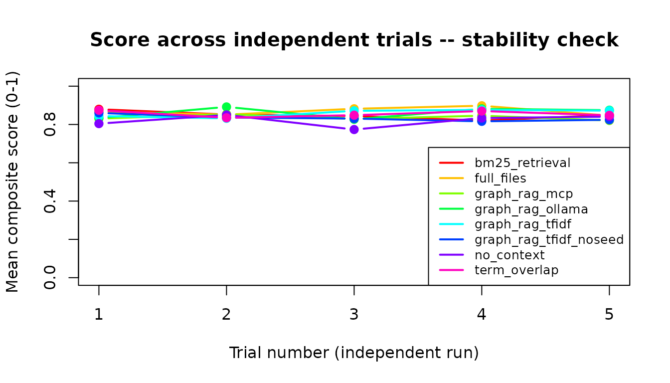
Score trajectory across trials
Each task is run n_trials times independently. If scores
improve across trials it suggests the LLM benefits from the specific
context being fed (learning effect within context window). Flat lines
indicate consistent performance; downward trends indicate
instability.
if (results_available && "trial" %in% names(all_results)) {
  trial_means <- aggregate(score ~ strategy + trial,
    data = all_results,
    FUN = function(x) mean(x, na.rm = TRUE)
  )
  strategies <- unique(trial_means$strategy)
  cols <- rainbow(length(strategies))
  plot(range(trial_means$trial), c(0, 1),
    type = "n",
    xlab = "Trial number (independent run)",
    ylab = "Mean composite score (0-1)",
    main = "Score across independent trials -- stability check"
  )
  for (i in seq_along(strategies)) {
    sub <- trial_means[trial_means$strategy == strategies[i], ]
    lines(sub$trial, sub$score, col = cols[i], lwd = 2, type = "b", pch = 19)
  }
  legend("bottomright", legend = strategies, col = cols, lwd = 2, cex = 0.8)
}
Session info
sessionInfo()
#> R version 4.5.3 (2026-03-11)
#> Platform: x86_64-pc-linux-gnu
#> Running under: Ubuntu 24.04.3 LTS
#>
#> Matrix products: default
#> BLAS:   /usr/lib/x86_64-linux-gnu/openblas-pthread/libblas.so.3
#> LAPACK: /usr/lib/x86_64-linux-gnu/openblas-pthread/libopenblasp-r0.3.26.so;  LAPACK version 3.12.0
#>
#> locale:
#>  [1] LC_CTYPE=C.UTF-8       LC_NUMERIC=C           LC_TIME=C.UTF-8
#>  [4] LC_COLLATE=C.UTF-8     LC_MONETARY=C.UTF-8    LC_MESSAGES=C.UTF-8
#>  [7] LC_PAPER=C.UTF-8       LC_NAME=C              LC_ADDRESS=C
#> [10] LC_TELEPHONE=C         LC_MEASUREMENT=C.UTF-8 LC_IDENTIFICATION=C
#>
#> time zone: UTC
#> tzcode source: system (glibc)
#>
#> attached base packages:
#> [1] stats     graphics  grDevices utils     datasets  methods   base
#>
#> other attached packages:
#> [1] rrlmgraphbench_0.1.3
#>
#> loaded via a namespace (and not attached):
#>  [1] digest_0.6.39     desc_1.4.3        R6_2.6.1          fastmap_1.2.0
#>  [5] xfun_0.57         cachem_1.1.0      knitr_1.51        htmltools_0.5.9
#>  [9] rmarkdown_2.30    lifecycle_1.0.5   cli_3.6.5         sass_0.4.10
#> [13] pkgdown_2.2.0     textshaping_1.0.5 jquerylib_0.1.4   systemfonts_1.3.2
#> [17] compiler_4.5.3    tools_4.5.3       ragg_1.5.1        bslib_0.10.0
#> [21] evaluate_1.0.5    yaml_2.3.12       otel_0.2.0        jsonlite_2.0.0
#> [25] rlang_1.1.7       fs_1.6.7          htmlwidgets_1.6.4