Annex. 1 Figures

Figure 1: Relation between IA-ML-DL
IA engloba a ML y ML engloba a DL

Taken from: Deep learning with R by Chollet and Allaire (2018).

Figure 2: Classic programming and machine learning
It shows a scheme that explains in a general way the paradigm of classical programming and the use of machine learning. Showing in the first how rules and data are entered to obtain answers, while in machine learning data and answers are entered to obtain rules

Taken from: Deep learning with R by Chollet and Allaire (2018).

Figure 3: Basic structure of an artificial neural network
Shows a schematic schematic of the basic structure of an RNA. It shows how the different inputs are connected to each of the hidden layer nodes and in turn how each of the hidden layer nodes is connected to the output layer nodes. The hidden layer and output layer nodes are also connected to a bias parameter

Taken from: Topic 14: neural networks of Larrañaga (2007).

Figure 4: How the size of the filter affects the output vector

Own elaboration: Elaborated from Jing (2020). Shows how the size of the output vector changes according to the size of the filter that is used.

Figure 5: How stride affects the output vector

Own elaboration: Elaborated from Jing (2020). Shows how the stride parameter affects the size of the output vector.

Figure 6: How dilation affects the output vector

Own elaboration: Elaborated from Jing (2020). Show how the dilation parameter affects the size of the output vector.

Figure 7: How padding affects the output vector

Own elaboration: Elaborated from Jing (2020). Show how the padding parameter affects the size of the output vector.

Figure 8: Deployment of the loop of a standard recurrent neural network

Taken from: Understanding LSTM networks, Olah (2015).

Figure 9: Nearby relevant information

Taken from: Understanding LSTM networks, Olah (2015).

Figure 10: Distant relevant information

Taken from: Understanding LSTM networks, Olah (2015).

Figure 11: Difference Between Repeat Modules

Taken from: Understanding LSTM networks, Olah (2015).

Figure 12: LSTM functionality: Representation of step 1

Taken from: Understanding LSTM networks, Olah (2015).

Figure 13: LSTM functionality: Representation of step 2

Taken from: Understanding LSTM networks, Olah (2015).

Figure 14: LSTM functionality: Representation of step 3

Taken from: Understanding LSTM networks, Olah (2015).

Figure 15: LSTM functionality: Representation of step 4

Taken from: Understanding LSTM networks, Olah (2015).

Figure 16: Input and output vector display

Own elaboration: Made from an image in Chollet and Allaire (2018). It shows what the three-dimensional input and output vectors for a company’s data look like, if three observations are used to create the input vector.

Figure 17: Different structures depending on the different sizes of input vectors

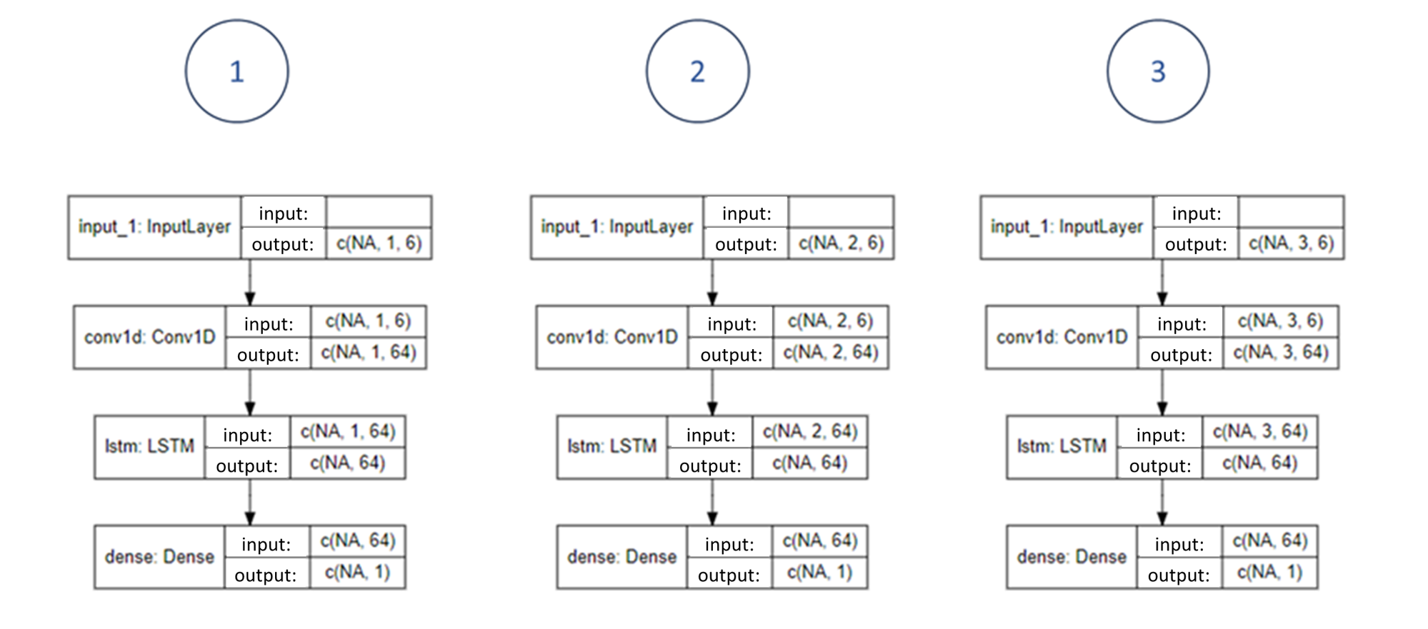
Own elaboration: Elaborated from the different models built using the keras and tensorflow packages in R and were graphed using the Iannone (2023) package.

Figure 18: ReLU and Leaky ReLU domain

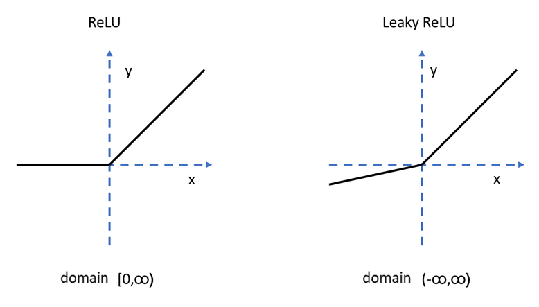
Own elaboration: Elaborated from the images that can be seen in Rallabandi (2023).
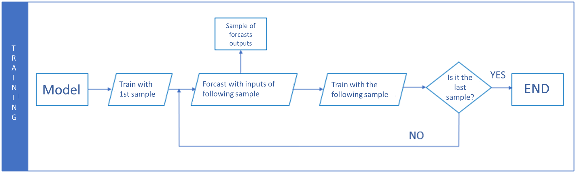
Figure 19: Flowchart of the Walk Forward Validation methodology

Own elaboration