Introduction
This vignette provides a comprehensive guide to using
kerasnip to define sequential Keras models within the
tidymodels ecosystem. kerasnip bridges the gap
between the imperative, layer-by-layer construction of Keras models and
the declarative, specification-based approach of
tidymodels.
Here, we will focus on create_keras_sequential_spec(),
which is ideal for models where layers form a plain stack, with each
layer having exactly one input tensor and one output tensor.
Setup
We’ll start by loading the necessary packages:
library(kerasnip)
library(tidymodels)
#> ── Attaching packages ────────────────────────────────────── tidymodels 1.5.0 ──
#> ✔ broom        1.0.13     ✔ recipes      1.3.3
#> ✔ dials        1.4.4      ✔ rsample      1.3.2
#> ✔ dplyr        1.2.1      ✔ tailor       0.1.0
#> ✔ ggplot2      4.0.3      ✔ tidyr        1.3.2
#> ✔ infer        1.1.0      ✔ tune         2.1.0
#> ✔ modeldata    1.5.1      ✔ workflows    1.3.0
#> ✔ parsnip      1.6.0      ✔ workflowsets 1.1.1
#> ✔ purrr        1.2.2      ✔ yardstick    1.4.0
#> ── Conflicts ───────────────────────────────────────── tidymodels_conflicts() ──
#> ✖ purrr::discard() masks scales::discard()
#> ✖ dplyr::filter()  masks stats::filter()
#> ✖ dplyr::lag()     masks stats::lag()
#> ✖ recipes::step()  masks stats::step()
library(keras3)
#>
#> Attaching package: 'keras3'
#> The following object is masked from 'package:yardstick':
#>
#>     get_weights
#> The following object is masked from 'package:infer':
#>
#>     generate
When to use create_keras_sequential_spec()
A Sequential model in Keras is appropriate for a plain
stack of layers where each layer has exactly one input tensor and one
output tensor. kerasnip’s
create_keras_sequential_spec() function is designed to
define such models in a tidymodels-compatible way.
Instead of building the model layer-by-layer imperatively, you define
a named, ordered list of R functions called layer_blocks.
Each layer_block function takes a Keras model object as its
first argument and returns the modified model. kerasnip
then uses these blocks to construct the full Keras Sequential model.
For models with more complex, non-linear topologies (e.g., multiple
inputs/outputs, residual connections, or multi-branch models), you
should use create_keras_functional_spec().
Creating a kerasnip Sequential Model Specification
Let’s define a simple sequential model with three dense layers.
First, we define our layer_blocks:
# The first block must initialize the model. `input_shape`
# is passed automatically.
input_block <- function(model, input_shape) {
  keras_model_sequential(input_shape = input_shape)
}

# A reusable block for hidden layers. `units` will become a tunable parameter.
hidden_block <- function(model, units = 32, activation = "relu") {
  model |> layer_dense(units = units, activation = activation)
}

# The output block. `num_classes` is passed automatically for classification.
output_block <- function(model, num_classes, activation = "softmax") {
  model |> layer_dense(units = num_classes, activation = activation)
}
Now, we use create_keras_sequential_spec() to generate
our parsnip model specification function. We’ll name our
model my_simple_mlp.
create_keras_sequential_spec(
  model_name = "my_simple_mlp",
  layer_blocks = list(
    input = input_block,
    hidden_1 = hidden_block,
    hidden_2 = hidden_block,
    output = output_block
  ),
  mode = "classification"
)
A common debugging workflow: compile_keras_grid()
In the original Keras guide, a common workflow is to incrementally
add layers and call summary() to inspect the architecture.
With kerasnip, the model is defined declaratively, so we
can’t inspect it layer-by-layer in the same way.
However, kerasnip provides a powerful equivalent:
compile_keras_grid(). This function checks if your
layer_blocks define a valid Keras model and returns the
compiled model structure, all without running a full training cycle.
This is perfect for debugging your architecture.
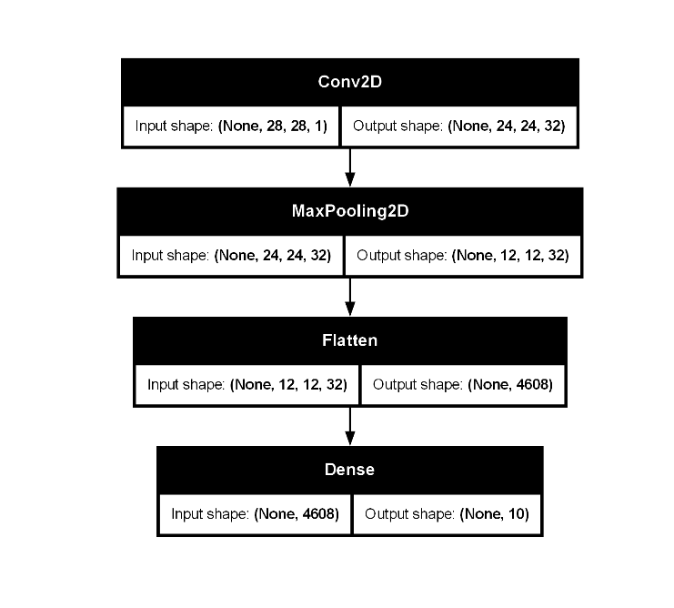
Let’s see this in action with a CNN architecture:
# Define CNN layer blocks
cnn_input_block <- function(model, input_shape) {
  keras_model_sequential(input_shape = input_shape)
}
cnn_conv_block <- function(
  model,
  filters = 32,
  kernel_size = 3,
  activation = "relu"
) {
  model |>
    layer_conv_2d(
      filters = filters,
      kernel_size = kernel_size,
      activation = activation
    )
}
cnn_pool_block <- function(model, pool_size = 2) {
  model |> layer_max_pooling_2d(pool_size = pool_size)
}
cnn_flatten_block <- function(model) {
  model |> layer_flatten()
}
cnn_output_block <- function(model, num_classes, activation = "softmax") {
  model |> layer_dense(units = num_classes, activation = activation)
}

# Create the kerasnip spec function
create_keras_sequential_spec(
  model_name = "my_cnn",
  layer_blocks = list(
    input = cnn_input_block,
    conv1 = cnn_conv_block,
    pool1 = cnn_pool_block,
    flatten = cnn_flatten_block,
    output = cnn_output_block
  ),
  mode = "classification"
)

# Create a spec instance for a 28x28x1 image
cnn_spec <- my_cnn(
  conv1_filters = 32, conv1_kernel_size = 5,
  compile_loss = "categorical_crossentropy",
  compile_optimizer = "adam"
)

# Prepare dummy data with the correct shape.
# We create a list of 28x28x1 arrays.
x_dummy_list <- lapply(
  1:10,
  function(i) array(runif(28 * 28 * 1), dim = c(28, 28, 1))
)
x_dummy_df <- tibble::tibble(x = x_dummy_list)
y_dummy <- factor(sample(0:9, 10, replace = TRUE), levels = 0:9)
y_dummy_df <- tibble::tibble(y = y_dummy)


# Use compile_keras_grid to get the model summary
# A one-row grid with no extra hyperparameters builds the spec as-is.
compilation_results <- compile_keras_grid(
  spec = cnn_spec,
  grid = tibble::tibble(.rows = 1L),
  x = x_dummy_df,
  y = y_dummy_df
)

# Print the summary
compilation_results |>
  select(compiled_model) |>
  pull() |>
  pluck(1) |>
  summary()
#> Model: "sequential"
#> ┏━━━━━━━━━━━━━━━━━━━━━━━━━━━━━━━━━━━┳━━━━━━━━━━━━━━━━━━━━━━━━━━┳━━━━━━━━━━━━━━━┓
#> ┃ Layer (type)                      ┃ Output Shape             ┃       Param # ┃
#> ┡━━━━━━━━━━━━━━━━━━━━━━━━━━━━━━━━━━━╇━━━━━━━━━━━━━━━━━━━━━━━━━━╇━━━━━━━━━━━━━━━┩
#> │ conv2d (Conv2D)                   │ (None, 24, 24, 32)       │           832 │
#> ├───────────────────────────────────┼──────────────────────────┼───────────────┤
#> │ max_pooling2d (MaxPooling2D)      │ (None, 12, 12, 32)       │             0 │
#> ├───────────────────────────────────┼──────────────────────────┼───────────────┤
#> │ flatten (Flatten)                 │ (None, 4608)             │             0 │
#> ├───────────────────────────────────┼──────────────────────────┼───────────────┤
#> │ dense (Dense)                     │ (None, 10)               │        46,090 │
#> └───────────────────────────────────┴──────────────────────────┴───────────────┘
#>  Total params: 46,922 (183.29 KB)
#>  Trainable params: 46,922 (183.29 KB)
#>  Non-trainable params: 0 (0.00 B)