Tidymodels Workflow with Functional Keras Models (Multi-Input)

Introduction

This vignette demonstrates a complete tidymodels workflow for a regression task using a Keras functional model defined with kerasnip. We will use the Ames Housing dataset to predict house prices. A key feature of this example is the use of a multi-input Keras model, where numerical and categorical features are processed through separate input branches.

kerasnip allows you to define complex Keras architectures, including those with multiple inputs, and integrate them seamlessly into the tidymodels ecosystem for robust modeling and tuning.

Setup

First, we load the necessary packages.

library(kerasnip)
library(tidymodels)
#> ── Attaching packages ────────────────────────────────────── tidymodels 1.3.0 ──
#> ✔ broom        1.0.9     ✔ recipes      1.3.1
#> ✔ dials        1.4.1     ✔ rsample      1.3.1
#> ✔ dplyr        1.1.4     ✔ tibble       3.3.0
#> ✔ ggplot2      3.5.2     ✔ tidyr        1.3.1
#> ✔ infer        1.0.9     ✔ tune         1.3.0
#> ✔ modeldata    1.5.1     ✔ workflows    1.2.0
#> ✔ parsnip      1.3.2     ✔ workflowsets 1.1.1
#> ✔ purrr        1.1.0     ✔ yardstick    1.3.2
#> ── Conflicts ───────────────────────────────────────── tidymodels_conflicts() ──
#> ✖ purrr::discard() masks scales::discard()
#> ✖ dplyr::filter()  masks stats::filter()
#> ✖ dplyr::lag()     masks stats::lag()
#> ✖ recipes::step()  masks stats::step()
library(keras3)
#> 
#> Attaching package: 'keras3'
#> The following object is masked from 'package:yardstick':
#> 
#>     get_weights
library(dplyr)       # For data manipulation
library(ggplot2)     # For plotting
library(future)      # For parallel processing
#> 
#> Attaching package: 'future'
#> The following object is masked from 'package:keras3':
#> 
#>     %<-%
library(finetune)    # For racing

Data Preparation

We’ll use the Ames Housing dataset, which is available in the modeldata package. We will then split the data into training and testing sets.

# Select relevant columns and remove rows with missing values
ames_df <- ames |>
  select(
    Sale_Price,
    Gr_Liv_Area,
    Year_Built,
    Neighborhood,
    Bldg_Type,
    Overall_Cond,
    Total_Bsmt_SF,
    contains("SF")
  ) |>
  na.omit()

# Split data into training and testing sets
set.seed(123)
ames_split <- initial_split(ames_df, prop = 0.8, strata = Sale_Price)
ames_train <- training(ames_split)
ames_test <- testing(ames_split)

# Create cross-validation folds for tuning
ames_folds <- vfold_cv(ames_train, v = 5, strata = Sale_Price)

Recipe for Preprocessing

We will create a recipes object to preprocess our data. This recipe will: * Predict Sale_Price using all other variables. * Normalize all numerical predictors. * Create dummy variables for categorical predictors. * Collapse each group of predictors into a single matrix column using step_collapse().

This final step is crucial for the multi-input Keras model, as the kerasnip functional API expects a list of matrices for multiple inputs, where each matrix corresponds to a distinct input layer.

ames_recipe <- recipe(Sale_Price ~ ., data = ames_train) |>
  step_normalize(all_numeric_predictors()) |>
  step_collapse(all_numeric_predictors(), new_col = "numerical_input") |>
  step_dummy(Neighborhood) |>
  step_collapse(starts_with("Neighborhood"), new_col = "neighborhood_input") |>
  step_dummy(Bldg_Type) |>
  step_collapse(starts_with("Bldg_Type"), new_col = "bldg_input") |>
  step_dummy(Overall_Cond) |>
  step_collapse(starts_with("Overall_Cond"), new_col = "condition_input")

Define Keras Functional Model with kerasnip

Now, we define our Keras functional model using kerasnip’s layer blocks. This model will have four distinct input layers: one for numerical features and three for categorical features. These branches will be processed separately and then concatenated before the final output layer.

# Define layer blocks for multi-input functional model

# Input blocks for numerical and categorical features
input_numerical <- function(input_shape) {
  layer_input(shape = input_shape, name = "numerical_input")
}

input_neighborhood <- function(input_shape) {
  layer_input(shape = input_shape, name = "neighborhood_input")
}

input_bldg <- function(input_shape) {
  layer_input(shape = input_shape, name = "bldg_input")
}

input_condition <- function(input_shape) {
  layer_input(shape = input_shape, name = "condition_input")
}

# Processing blocks for each input type
dense_numerical <- function(tensor, units = 32, activation = "relu") {
  tensor |>
    layer_dense(units = units, activation = activation)
}

dense_categorical <- function(tensor, units = 16, activation = "relu") {
  tensor |>
    layer_dense(units = units, activation = activation)
}

# Concatenation block
concatenate_features <- function(numeric, neighborhood, bldg, condition) {
  layer_concatenate(list(numeric, neighborhood, bldg, condition))
}

# Output block for regression
output_regression <- function(tensor) {
  layer_dense(tensor, units = 1, name = "output")
}

# Create the kerasnip model specification function
create_keras_functional_spec(
  model_name = "ames_functional_mlp",
  layer_blocks = list(
    numerical_input = input_numerical,
    neighborhood_input = input_neighborhood,
    bldg_input = input_bldg,
    condition_input = input_condition,
    processed_numerical = inp_spec(dense_numerical, "numerical_input"),
    processed_neighborhood = inp_spec(dense_categorical, "neighborhood_input"),
    processed_bldg = inp_spec(dense_categorical, "bldg_input"),
    processed_condition = inp_spec(dense_categorical, "condition_input"),
    combined_features = inp_spec(
      concatenate_features,
      c(
        processed_numerical = "numeric",
        processed_neighborhood = "neighborhood",
        processed_bldg = "bldg",
        processed_condition = "condition"
      )
    ),
    output = inp_spec(output_regression, "combined_features")
  ),
  mode = "regression"
)

Model Specification

We’ll define our ames_functional_mlp model specification and set some hyperparameters to tune(). Note how the arguments are prefixed with their corresponding block names (e.g., processed_numerical_units).

# Define the tunable model specification
functional_mlp_spec <- ames_functional_mlp(
  # Tunable parameters for numerical branch
  processed_numerical_units = tune(),
  # Tunable parameters for categorical branch
  processed_neighborhood_units = tune(),
  processed_bldg_units = tune(),
  processed_condition_units = tune(),
  # Fixed compilation and fitting parameters
  compile_loss = "mean_squared_error",
  compile_optimizer = "adam",
  compile_metrics = c("mean_absolute_error"),
  fit_epochs = 50,
  fit_batch_size = 32,
  fit_validation_split = 0.2,
  fit_callbacks = list(
    callback_early_stopping(monitor = "val_loss", patience = 5)
  )
) |>
  set_engine("keras")

print(functional_mlp_spec)
#> ames functional mlp Model Specification (regression)
#> 
#> Main Arguments:
#>   num_numerical_input = structure(list(), class = "rlang_zap")
#>   num_neighborhood_input = structure(list(), class = "rlang_zap")
#>   num_bldg_input = structure(list(), class = "rlang_zap")
#>   num_condition_input = structure(list(), class = "rlang_zap")
#>   num_processed_numerical = structure(list(), class = "rlang_zap")
#>   num_processed_neighborhood = structure(list(), class = "rlang_zap")
#>   num_processed_bldg = structure(list(), class = "rlang_zap")
#>   num_processed_condition = structure(list(), class = "rlang_zap")
#>   num_combined_features = structure(list(), class = "rlang_zap")
#>   num_output = structure(list(), class = "rlang_zap")
#>   processed_numerical_units = tune()
#>   processed_numerical_activation = structure(list(), class = "rlang_zap")
#>   processed_neighborhood_units = tune()
#>   processed_neighborhood_activation = structure(list(), class = "rlang_zap")
#>   processed_bldg_units = tune()
#>   processed_bldg_activation = structure(list(), class = "rlang_zap")
#>   processed_condition_units = tune()
#>   processed_condition_activation = structure(list(), class = "rlang_zap")
#>   learn_rate = structure(list(), class = "rlang_zap")
#>   fit_batch_size = 32
#>   fit_epochs = 50
#>   fit_callbacks = list(callback_early_stopping(monitor = "val_loss", patience = 5))
#>   fit_validation_split = 0.2
#>   fit_validation_data = structure(list(), class = "rlang_zap")
#>   fit_shuffle = structure(list(), class = "rlang_zap")
#>   fit_class_weight = structure(list(), class = "rlang_zap")
#>   fit_sample_weight = structure(list(), class = "rlang_zap")
#>   fit_initial_epoch = structure(list(), class = "rlang_zap")
#>   fit_steps_per_epoch = structure(list(), class = "rlang_zap")
#>   fit_validation_steps = structure(list(), class = "rlang_zap")
#>   fit_validation_batch_size = structure(list(), class = "rlang_zap")
#>   fit_validation_freq = structure(list(), class = "rlang_zap")
#>   fit_verbose = structure(list(), class = "rlang_zap")
#>   fit_view_metrics = structure(list(), class = "rlang_zap")
#>   compile_optimizer = adam
#>   compile_loss = mean_squared_error
#>   compile_metrics = c("mean_absolute_error")
#>   compile_loss_weights = structure(list(), class = "rlang_zap")
#>   compile_weighted_metrics = structure(list(), class = "rlang_zap")
#>   compile_run_eagerly = structure(list(), class = "rlang_zap")
#>   compile_steps_per_execution = structure(list(), class = "rlang_zap")
#>   compile_jit_compile = structure(list(), class = "rlang_zap")
#>   compile_auto_scale_loss = structure(list(), class = "rlang_zap")
#> 
#> Computational engine: keras

Create Workflow

A workflow combines the recipe and the model specification.

ames_wf <- workflow() |>
  add_recipe(ames_recipe) |>
  add_model(functional_mlp_spec)

print(ames_wf)
#> ══ Workflow ════════════════════════════════════════════════════════════════════
#> Preprocessor: Recipe
#> Model: ames_functional_mlp()
#> 
#> ── Preprocessor ────────────────────────────────────────────────────────────────
#> 8 Recipe Steps
#> 
#> • step_normalize()
#> • step_collapse()
#> • step_dummy()
#> • step_collapse()
#> • step_dummy()
#> • step_collapse()
#> • step_dummy()
#> • step_collapse()
#> 
#> ── Model ───────────────────────────────────────────────────────────────────────
#> ames functional mlp Model Specification (regression)
#> 
#> Main Arguments:
#>   num_numerical_input = structure(list(), class = "rlang_zap")
#>   num_neighborhood_input = structure(list(), class = "rlang_zap")
#>   num_bldg_input = structure(list(), class = "rlang_zap")
#>   num_condition_input = structure(list(), class = "rlang_zap")
#>   num_processed_numerical = structure(list(), class = "rlang_zap")
#>   num_processed_neighborhood = structure(list(), class = "rlang_zap")
#>   num_processed_bldg = structure(list(), class = "rlang_zap")
#>   num_processed_condition = structure(list(), class = "rlang_zap")
#>   num_combined_features = structure(list(), class = "rlang_zap")
#>   num_output = structure(list(), class = "rlang_zap")
#>   processed_numerical_units = tune()
#>   processed_numerical_activation = structure(list(), class = "rlang_zap")
#>   processed_neighborhood_units = tune()
#>   processed_neighborhood_activation = structure(list(), class = "rlang_zap")
#>   processed_bldg_units = tune()
#>   processed_bldg_activation = structure(list(), class = "rlang_zap")
#>   processed_condition_units = tune()
#>   processed_condition_activation = structure(list(), class = "rlang_zap")
#>   learn_rate = structure(list(), class = "rlang_zap")
#>   fit_batch_size = 32
#>   fit_epochs = 50
#>   fit_callbacks = list(callback_early_stopping(monitor = "val_loss", patience = 5))
#>   fit_validation_split = 0.2
#>   fit_validation_data = structure(list(), class = "rlang_zap")
#>   fit_shuffle = structure(list(), class = "rlang_zap")
#>   fit_class_weight = structure(list(), class = "rlang_zap")
#>   fit_sample_weight = structure(list(), class = "rlang_zap")
#>   fit_initial_epoch = structure(list(), class = "rlang_zap")
#>   fit_steps_per_epoch = structure(list(), class = "rlang_zap")
#>   fit_validation_steps = structure(list(), class = "rlang_zap")
#>   fit_validation_batch_size = structure(list(), class = "rlang_zap")
#>   fit_validation_freq = structure(list(), class = "rlang_zap")
#>   fit_verbose = structure(list(), class = "rlang_zap")
#>   fit_view_metrics = structure(list(), class = "rlang_zap")
#>   compile_optimizer = adam
#>   compile_loss = mean_squared_error
#>   compile_metrics = c("mean_absolute_error")
#>   compile_loss_weights = structure(list(), class = "rlang_zap")
#>   compile_weighted_metrics = structure(list(), class = "rlang_zap")
#>   compile_run_eagerly = structure(list(), class = "rlang_zap")
#>   compile_steps_per_execution = structure(list(), class = "rlang_zap")
#>   compile_jit_compile = structure(list(), class = "rlang_zap")
#>   compile_auto_scale_loss = structure(list(), class = "rlang_zap")
#> 
#> Computational engine: keras

Define Tuning Grid

We will create a regular grid for our hyperparameters.

# Define the tuning grid
params <- extract_parameter_set_dials(ames_wf) |>
  update(
    processed_numerical_units = hidden_units(range = c(32, 128)),
    processed_neighborhood_units = hidden_units(range = c(16, 64)),
    processed_bldg_units = hidden_units(range = c(16, 64)),
    processed_condition_units = hidden_units(range = c(16, 64))
  )
functional_mlp_grid <- grid_regular(params, levels = 3)

print(functional_mlp_grid)
#> # A tibble: 81 × 4
#>    processed_numerical_units processed_neighborhood_units processed_bldg_units
#>                        <int>                        <int>                <int>
#>  1                        32                           16                   16
#>  2                        80                           16                   16
#>  3                       128                           16                   16
#>  4                        32                           40                   16
#>  5                        80                           40                   16
#>  6                       128                           40                   16
#>  7                        32                           64                   16
#>  8                        80                           64                   16
#>  9                       128                           64                   16
#> 10                        32                           16                   40
#> # ℹ 71 more rows
#> # ℹ 1 more variable: processed_condition_units <int>

Tune Model

Now, we’ll use tune_race_anova() to perform cross-validation and find the best hyperparameters.

# Note: Parallel processing with `plan(multisession)` is currently not working
# with Keras models due to backend conflicts

set.seed(123)
ames_tune_results <- tune_race_anova(
  ames_wf,
  resamples = ames_folds,
  grid = functional_mlp_grid,
  metrics = metric_set(rmse, mae, rsq),
  control = control_race(save_pred = TRUE, save_workflow = TRUE)
)
#> 15/15 - 0s - 6ms/step
#> 15/15 - 0s - 6ms/step
#> 15/15 - 0s - 6ms/step
#> 15/15 - 0s - 6ms/step
#> 15/15 - 0s - 6ms/step
#> 15/15 - 0s - 6ms/step
#> 15/15 - 0s - 6ms/step
#> 15/15 - 0s - 6ms/step
#> 15/15 - 0s - 6ms/step
#> 15/15 - 0s - 6ms/step
#> 15/15 - 0s - 6ms/step
#> 15/15 - 0s - 6ms/step
#> 15/15 - 0s - 6ms/step
#> 15/15 - 0s - 6ms/step
#> 15/15 - 0s - 6ms/step
#> 15/15 - 0s - 6ms/step
#> 15/15 - 0s - 6ms/step
#> 15/15 - 0s - 6ms/step
#> 15/15 - 0s - 6ms/step
#> 15/15 - 0s - 6ms/step
#> 15/15 - 0s - 6ms/step
#> 15/15 - 0s - 6ms/step
#> 15/15 - 0s - 6ms/step
#> 15/15 - 0s - 6ms/step
#> 15/15 - 0s - 6ms/step
#> 15/15 - 0s - 6ms/step
#> 15/15 - 0s - 6ms/step
#> 15/15 - 0s - 6ms/step
#> 15/15 - 0s - 6ms/step
#> 15/15 - 0s - 6ms/step
#> 15/15 - 0s - 6ms/step
#> 15/15 - 0s - 6ms/step
#> 15/15 - 0s - 6ms/step
#> 15/15 - 0s - 6ms/step
#> 15/15 - 0s - 6ms/step
#> 15/15 - 0s - 6ms/step
#> 15/15 - 0s - 6ms/step
#> 15/15 - 0s - 6ms/step
#> 15/15 - 0s - 6ms/step
#> 15/15 - 0s - 6ms/step
#> 15/15 - 0s - 6ms/step
#> 15/15 - 0s - 6ms/step
#> 15/15 - 0s - 6ms/step
#> 15/15 - 0s - 6ms/step
#> 15/15 - 0s - 6ms/step
#> 15/15 - 0s - 6ms/step
#> 15/15 - 0s - 6ms/step
#> 15/15 - 0s - 6ms/step
#> 15/15 - 0s - 6ms/step
#> 15/15 - 0s - 6ms/step
#> 15/15 - 0s - 6ms/step
#> 15/15 - 0s - 6ms/step
#> 15/15 - 0s - 6ms/step
#> 15/15 - 0s - 6ms/step
#> 15/15 - 0s - 6ms/step
#> 15/15 - 0s - 6ms/step
#> 15/15 - 0s - 6ms/step
#> 15/15 - 0s - 6ms/step
#> 15/15 - 0s - 6ms/step
#> 15/15 - 0s - 6ms/step
#> 15/15 - 0s - 6ms/step
#> 15/15 - 0s - 7ms/step
#> 15/15 - 0s - 7ms/step
#> 15/15 - 0s - 6ms/step
#> 15/15 - 0s - 7ms/step
#> 15/15 - 0s - 6ms/step
#> 15/15 - 0s - 6ms/step
#> 15/15 - 0s - 6ms/step
#> 15/15 - 0s - 6ms/step
#> 15/15 - 0s - 6ms/step
#> 15/15 - 0s - 6ms/step
#> 15/15 - 0s - 6ms/step
#> 15/15 - 0s - 6ms/step
#> 15/15 - 0s - 6ms/step
#> 15/15 - 0s - 6ms/step
#> 15/15 - 0s - 6ms/step
#> 15/15 - 0s - 6ms/step
#> 15/15 - 0s - 6ms/step
#> 15/15 - 0s - 7ms/step
#> 15/15 - 0s - 6ms/step
#> 15/15 - 0s - 6ms/step
#> 15/15 - 0s - 6ms/step
#> 15/15 - 0s - 6ms/step
#> 15/15 - 0s - 6ms/step
#> 15/15 - 0s - 6ms/step
#> 15/15 - 0s - 6ms/step
#> 15/15 - 0s - 6ms/step
#> 15/15 - 0s - 6ms/step
#> 15/15 - 0s - 6ms/step
#> 15/15 - 0s - 6ms/step
#> 15/15 - 0s - 6ms/step
#> 15/15 - 0s - 6ms/step
#> 15/15 - 0s - 6ms/step
#> 15/15 - 0s - 6ms/step
#> 15/15 - 0s - 6ms/step
#> 15/15 - 0s - 6ms/step
#> 15/15 - 0s - 6ms/step
#> 15/15 - 0s - 6ms/step
#> 15/15 - 0s - 6ms/step
#> 15/15 - 0s - 6ms/step
#> 15/15 - 0s - 6ms/step
#> 15/15 - 0s - 6ms/step
#> 15/15 - 0s - 6ms/step
#> 15/15 - 0s - 6ms/step
#> 15/15 - 0s - 6ms/step
#> 15/15 - 0s - 6ms/step
#> 15/15 - 0s - 6ms/step
#> 15/15 - 0s - 6ms/step
#> 15/15 - 0s - 7ms/step
#> 15/15 - 0s - 6ms/step
#> 15/15 - 0s - 6ms/step
#> 15/15 - 0s - 6ms/step
#> 15/15 - 0s - 6ms/step
#> 15/15 - 0s - 6ms/step
#> 15/15 - 0s - 6ms/step
#> 15/15 - 0s - 6ms/step
#> 15/15 - 0s - 7ms/step
#> 15/15 - 0s - 7ms/step
#> 15/15 - 0s - 7ms/step
#> 15/15 - 0s - 6ms/step
#> 15/15 - 0s - 6ms/step
#> 15/15 - 0s - 6ms/step
#> 15/15 - 0s - 6ms/step
#> 15/15 - 0s - 6ms/step
#> 15/15 - 0s - 6ms/step
#> 15/15 - 0s - 6ms/step
#> 15/15 - 0s - 6ms/step
#> 15/15 - 0s - 6ms/step
#> 15/15 - 0s - 6ms/step
#> 15/15 - 0s - 6ms/step
#> 15/15 - 0s - 6ms/step
#> 15/15 - 0s - 6ms/step
#> 15/15 - 0s - 6ms/step
#> 15/15 - 0s - 6ms/step
#> 15/15 - 0s - 6ms/step
#> 15/15 - 0s - 6ms/step
#> 15/15 - 0s - 6ms/step
#> 15/15 - 0s - 6ms/step
#> 15/15 - 0s - 6ms/step
#> 15/15 - 0s - 6ms/step
#> 15/15 - 0s - 7ms/step
#> 15/15 - 0s - 7ms/step
#> 15/15 - 0s - 6ms/step
#> 15/15 - 0s - 6ms/step
#> 15/15 - 0s - 6ms/step
#> 15/15 - 0s - 6ms/step
#> 15/15 - 0s - 6ms/step
#> 15/15 - 0s - 6ms/step
#> 15/15 - 0s - 6ms/step
#> 15/15 - 0s - 6ms/step
#> 15/15 - 0s - 6ms/step
#> 15/15 - 0s - 6ms/step
#> 15/15 - 0s - 6ms/step
#> 15/15 - 0s - 6ms/step
#> 15/15 - 0s - 6ms/step
#> 15/15 - 0s - 6ms/step
#> 15/15 - 0s - 6ms/step
#> 15/15 - 0s - 6ms/step
#> 15/15 - 0s - 6ms/step
#> 15/15 - 0s - 6ms/step
#> 15/15 - 0s - 6ms/step
#> 15/15 - 0s - 6ms/step
#> 15/15 - 0s - 6ms/step
#> 15/15 - 0s - 6ms/step
#> 15/15 - 0s - 6ms/step
#> 15/15 - 0s - 6ms/step
#> 15/15 - 0s - 6ms/step
#> 15/15 - 0s - 6ms/step
#> 15/15 - 0s - 6ms/step
#> 15/15 - 0s - 7ms/step
#> 15/15 - 0s - 6ms/step
#> 15/15 - 0s - 6ms/step
#> 15/15 - 0s - 6ms/step
#> 15/15 - 0s - 6ms/step
#> 15/15 - 0s - 6ms/step
#> 15/15 - 0s - 6ms/step
#> 15/15 - 0s - 6ms/step
#> 15/15 - 0s - 6ms/step
#> 15/15 - 0s - 6ms/step
#> 15/15 - 0s - 6ms/step
#> 15/15 - 0s - 6ms/step
#> 15/15 - 0s - 6ms/step
#> 15/15 - 0s - 6ms/step
#> 15/15 - 0s - 6ms/step
#> 15/15 - 0s - 6ms/step
#> 15/15 - 0s - 6ms/step
#> 15/15 - 0s - 6ms/step
#> 15/15 - 0s - 6ms/step
#> 15/15 - 0s - 6ms/step
#> 15/15 - 0s - 6ms/step
#> 15/15 - 0s - 6ms/step
#> 15/15 - 0s - 6ms/step
#> 15/15 - 0s - 6ms/step
#> 15/15 - 0s - 6ms/step
#> 15/15 - 0s - 6ms/step
#> 15/15 - 0s - 6ms/step
#> 15/15 - 0s - 6ms/step
#> 15/15 - 0s - 6ms/step
#> 15/15 - 0s - 6ms/step
#> 15/15 - 0s - 6ms/step
#> 15/15 - 0s - 6ms/step
#> 15/15 - 0s - 6ms/step
#> 15/15 - 0s - 6ms/step
#> 15/15 - 0s - 7ms/step
#> 15/15 - 0s - 6ms/step
#> 15/15 - 0s - 7ms/step
#> 15/15 - 0s - 7ms/step
#> 15/15 - 0s - 6ms/step
#> 15/15 - 0s - 7ms/step
#> 15/15 - 0s - 6ms/step
#> 15/15 - 0s - 6ms/step
#> 15/15 - 0s - 6ms/step
#> 15/15 - 0s - 7ms/step
#> 15/15 - 0s - 6ms/step
#> 15/15 - 0s - 6ms/step
#> 15/15 - 0s - 6ms/step
#> 15/15 - 0s - 6ms/step
#> 15/15 - 0s - 6ms/step
#> 15/15 - 0s - 6ms/step
#> 15/15 - 0s - 6ms/step
#> 15/15 - 0s - 6ms/step
#> 15/15 - 0s - 6ms/step
#> 15/15 - 0s - 6ms/step
#> 15/15 - 0s - 6ms/step
#> 15/15 - 0s - 6ms/step
#> 15/15 - 0s - 6ms/step
#> 15/15 - 0s - 6ms/step
#> 15/15 - 0s - 6ms/step
#> 15/15 - 0s - 6ms/step
#> 15/15 - 0s - 6ms/step
#> 15/15 - 0s - 6ms/step
#> 15/15 - 0s - 6ms/step
#> 15/15 - 0s - 6ms/step
#> 15/15 - 0s - 6ms/step
#> 15/15 - 0s - 6ms/step
#> 15/15 - 0s - 6ms/step
#> 15/15 - 0s - 6ms/step
#> 15/15 - 0s - 6ms/step
#> 15/15 - 0s - 6ms/step
#> 15/15 - 0s - 6ms/step
#> 15/15 - 0s - 6ms/step
#> 15/15 - 0s - 6ms/step
#> 15/15 - 0s - 7ms/step
#> 15/15 - 0s - 7ms/step
#> 15/15 - 0s - 6ms/step
#> 15/15 - 0s - 6ms/step
#> 15/15 - 0s - 6ms/step
#> 15/15 - 0s - 6ms/step
#> 15/15 - 0s - 6ms/step
#> 15/15 - 0s - 7ms/step
#> 15/15 - 0s - 7ms/step
#> 15/15 - 0s - 7ms/step
#> 15/15 - 0s - 6ms/step
#> 15/15 - 0s - 6ms/step
#> 15/15 - 0s - 6ms/step
#> 15/15 - 0s - 6ms/step
#> 15/15 - 0s - 6ms/step

Inspect Tuning Results

We can inspect the tuning results to see which hyperparameter combinations performed best.

# Show the best performing models based on RMSE
show_best(ames_tune_results, metric = "rmse", n = 5)
#> # A tibble: 1 × 10
#>   processed_numerical_units processed_neighborhood_units processed_bldg_units
#>                       <int>                        <int>                <int>
#> 1                       128                           64                   64
#> # ℹ 7 more variables: processed_condition_units <int>, .metric <chr>,
#> #   .estimator <chr>, mean <dbl>, n <int>, std_err <dbl>, .config <chr>

# Autoplot the results
# Currently does not work due to a label issue: autoplot(ames_tune_results)

# Select the best hyperparameters
best_functional_mlp_params <- select_best(ames_tune_results, metric = "rmse")
print(best_functional_mlp_params)
#> # A tibble: 1 × 5
#>   processed_numerical_units processed_neighborhood_units processed_bldg_units
#>                       <int>                        <int>                <int>
#> 1                       128                           64                   64
#> # ℹ 2 more variables: processed_condition_units <int>, .config <chr>

Finalize Workflow and Fit Model

Once we have the best hyperparameters, we finalize the workflow and fit the model on the entire training dataset.

# Finalize the workflow with the best hyperparameters
final_ames_wf <- finalize_workflow(ames_wf, best_functional_mlp_params)

# Fit the final model on the full training data
final_ames_fit <- fit(final_ames_wf, data = ames_train)

print(final_ames_fit)
#> ══ Workflow [trained] ══════════════════════════════════════════════════════════
#> Preprocessor: Recipe
#> Model: ames_functional_mlp()
#> 
#> ── Preprocessor ────────────────────────────────────────────────────────────────
#> 8 Recipe Steps
#> 
#> • step_normalize()
#> • step_collapse()
#> • step_dummy()
#> • step_collapse()
#> • step_dummy()
#> • step_collapse()
#> • step_dummy()
#> • step_collapse()
#> 
#> ── Model ───────────────────────────────────────────────────────────────────────
#> $fit
#> Model: "functional_257"
#> ┏━━━━━━━━━━━━━━━━━━━━━━━┳━━━━━━━━━━━━━━━━━━━┳━━━━━━━━━━━━━┳━━━━━━━━━━━━━━━━━━━━┓
#> ┃ Layer (type)          ┃ Output Shape      ┃     Param # ┃ Connected to       ┃
#> ┡━━━━━━━━━━━━━━━━━━━━━━━╇━━━━━━━━━━━━━━━━━━━╇━━━━━━━━━━━━━╇━━━━━━━━━━━━━━━━━━━━┩
#> │ numerical_input       │ (None, 1, 10)     │           0 │ -                  │
#> │ (InputLayer)          │                   │             │                    │
#> ├───────────────────────┼───────────────────┼─────────────┼────────────────────┤
#> │ neighborhood_input    │ (None, 1, 28)     │           0 │ -                  │
#> │ (InputLayer)          │                   │             │                    │
#> ├───────────────────────┼───────────────────┼─────────────┼────────────────────┤
#> │ bldg_input            │ (None, 1, 4)      │           0 │ -                  │
#> │ (InputLayer)          │                   │             │                    │
#> ├───────────────────────┼───────────────────┼─────────────┼────────────────────┤
#> │ condition_input       │ (None, 1, 9)      │           0 │ -                  │
#> │ (InputLayer)          │                   │             │                    │
#> ├───────────────────────┼───────────────────┼─────────────┼────────────────────┤
#> │ dense_1028 (Dense)    │ (None, 1, 128)    │       1,408 │ numerical_input[0… │
#> ├───────────────────────┼───────────────────┼─────────────┼────────────────────┤
#> │ dense_1029 (Dense)    │ (None, 1, 64)     │       1,856 │ neighborhood_inpu… │
#> ├───────────────────────┼───────────────────┼─────────────┼────────────────────┤
#> │ dense_1030 (Dense)    │ (None, 1, 64)     │         320 │ bldg_input[0][0]   │
#> ├───────────────────────┼───────────────────┼─────────────┼────────────────────┤
#> │ dense_1031 (Dense)    │ (None, 1, 64)     │         640 │ condition_input[0… │
#> ├───────────────────────┼───────────────────┼─────────────┼────────────────────┤
#> │ concatenate_257       │ (None, 1, 320)    │           0 │ dense_1028[0][0],  │
#> │ (Concatenate)         │                   │             │ dense_1029[0][0],  │
#> │                       │                   │             │ dense_1030[0][0],  │
#> │                       │                   │             │ dense_1031[0][0]   │
#> ├───────────────────────┼───────────────────┼─────────────┼────────────────────┤
#> │ output (Dense)        │ (None, 1, 1)      │         321 │ concatenate_257[0… │
#> └───────────────────────┴───────────────────┴─────────────┴────────────────────┘
#>  Total params: 13,637 (53.27 KB)
#>  Trainable params: 4,545 (17.75 KB)
#>  Non-trainable params: 0 (0.00 B)
#>  Optimizer params: 9,092 (35.52 KB)
#> 
#> $history
#> 
#> Final epoch (plot to see history):
#>                    loss: 1,172,156,160
#>     mean_absolute_error: 21,003
#>                val_loss: 6,177,500,672
#> val_mean_absolute_error: 59,756 
#> 
#> $lvl
#> NULL
#> 
#> $process_x
#> function (x) 
#> 
#> ...
#> and 88 more lines.

Inspect Final Model

You can extract the underlying Keras model and its training history for further inspection.

# Extract the Keras model summary
final_ames_fit |>
  extract_fit_parsnip() |>
  extract_keras_model() |>
  summary()
#> Model: "functional_257"
#> ┏━━━━━━━━━━━━━━━━━━━━━━━┳━━━━━━━━━━━━━━━━━━━┳━━━━━━━━━━━━━┳━━━━━━━━━━━━━━━━━━━━┓
#> ┃ Layer (type)          ┃ Output Shape      ┃     Param # ┃ Connected to       ┃
#> ┡━━━━━━━━━━━━━━━━━━━━━━━╇━━━━━━━━━━━━━━━━━━━╇━━━━━━━━━━━━━╇━━━━━━━━━━━━━━━━━━━━┩
#> │ numerical_input       │ (None, 1, 10)     │           0 │ -                  │
#> │ (InputLayer)          │                   │             │                    │
#> ├───────────────────────┼───────────────────┼─────────────┼────────────────────┤
#> │ neighborhood_input    │ (None, 1, 28)     │           0 │ -                  │
#> │ (InputLayer)          │                   │             │                    │
#> ├───────────────────────┼───────────────────┼─────────────┼────────────────────┤
#> │ bldg_input            │ (None, 1, 4)      │           0 │ -                  │
#> │ (InputLayer)          │                   │             │                    │
#> ├───────────────────────┼───────────────────┼─────────────┼────────────────────┤
#> │ condition_input       │ (None, 1, 9)      │           0 │ -                  │
#> │ (InputLayer)          │                   │             │                    │
#> ├───────────────────────┼───────────────────┼─────────────┼────────────────────┤
#> │ dense_1028 (Dense)    │ (None, 1, 128)    │       1,408 │ numerical_input[0… │
#> ├───────────────────────┼───────────────────┼─────────────┼────────────────────┤
#> │ dense_1029 (Dense)    │ (None, 1, 64)     │       1,856 │ neighborhood_inpu… │
#> ├───────────────────────┼───────────────────┼─────────────┼────────────────────┤
#> │ dense_1030 (Dense)    │ (None, 1, 64)     │         320 │ bldg_input[0][0]   │
#> ├───────────────────────┼───────────────────┼─────────────┼────────────────────┤
#> │ dense_1031 (Dense)    │ (None, 1, 64)     │         640 │ condition_input[0… │
#> ├───────────────────────┼───────────────────┼─────────────┼────────────────────┤
#> │ concatenate_257       │ (None, 1, 320)    │           0 │ dense_1028[0][0],  │
#> │ (Concatenate)         │                   │             │ dense_1029[0][0],  │
#> │                       │                   │             │ dense_1030[0][0],  │
#> │                       │                   │             │ dense_1031[0][0]   │
#> ├───────────────────────┼───────────────────┼─────────────┼────────────────────┤
#> │ output (Dense)        │ (None, 1, 1)      │         321 │ concatenate_257[0… │
#> └───────────────────────┴───────────────────┴─────────────┴────────────────────┘
#>  Total params: 13,637 (53.27 KB)
#>  Trainable params: 4,545 (17.75 KB)
#>  Non-trainable params: 0 (0.00 B)
#>  Optimizer params: 9,092 (35.52 KB)

# Plot the Keras model
final_ames_fit |>
  extract_fit_parsnip() |>
  extract_keras_model() |>
  plot(show_shapes = TRUE)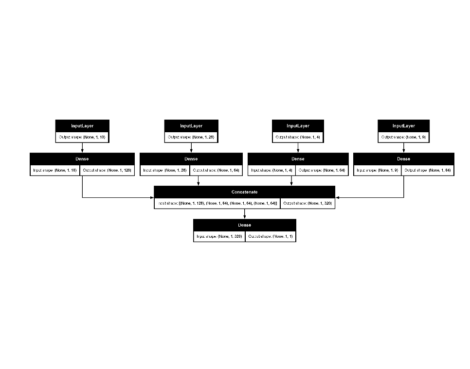

Model

# Plot the training history
final_ames_fit |>
  extract_fit_parsnip() |>
  extract_keras_history() |>
  plot()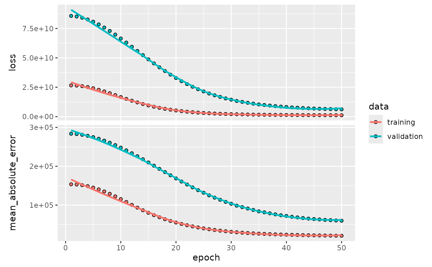

Make Predictions and Evaluate

Finally, we will make predictions on the test set and evaluate the model’s performance.

# Make predictions on the test set
ames_test_pred <- predict(final_ames_fit, new_data = ames_test)
#> 19/19 - 0s - 5ms/step

# Combine predictions with actuals
ames_results <- tibble::tibble(
  Sale_Price = ames_test$Sale_Price,
  .pred = ames_test_pred$.pred
)

print(head(ames_results))
#> # A tibble: 6 × 2
#>   Sale_Price   .pred
#>        <int>   <dbl>
#> 1     105000  97384.
#> 2     172000 163307.
#> 3     189900 193412.
#> 4     115000 126270.
#> 5     395192 265886.
#> 6     214000 214812.

# Evaluate performance using yardstick metrics
metrics_results <- metric_set(
  rmse,
  mae,
  rsq
)(
  ames_results,
  truth = Sale_Price,
  estimate = .pred
)

print(metrics_results)
#> # A tibble: 3 × 3
#>   .metric .estimator .estimate
#>   <chr>   <chr>          <dbl>
#> 1 rmse    standard   50898.   
#> 2 mae     standard   30777.   
#> 3 rsq     standard       0.786