Multi-Step Time Series Forecasting with kerasnip • kerasnip

This vignette shows how to build a Keras recurrent model with kerasnip that forecasts several future steps of a time series at once, using the “single-shot” multi-step pattern from Keras/TensorFlow’s own time series forecasting tutorial, adapted to the tidymodels ecosystem.

The Building Blocks

Two ingredients turn flat, ordered tabular data into the shapes an RNN-based forecaster needs:

step_sequence() slides a window of timesteps past rows into a single list-column of (timesteps, features) matrices: the (samples, timesteps, features) shape keras3::layer_lstm() / keras3::layer_gru() expect as input.
step_lead() builds the forecast target: one column per future step (lead_1_<var>, lead_2_<var>, …). Unlike recipes::step_lag(), which only supports past shifts, step_lead() shifts forward, which is what a multi-step-ahead target needs.

When both steps draw on the same raw column, step_lead() must come first: step_sequence() consumes (and drops) its source column once it has built the window, so step_lead() needs to see the raw column while it still exists.

The resulting outcome columns (lead_1_<var>, lead_2_<var>, …) are all numeric and map to a single output block sized units = horizon: one Keras output node predicting the whole vector of future values in one forward pass, sharing one loss. This is different from the multi-output models in vignette("functional_api"), where each outcome column becomes its own independently-configured head; here there is only one output block, so kerasnip packs the numeric outcome columns into a single (samples, horizon) matrix target instead of splitting them.

Step 1: Load Libraries and Simulate a Series

library(kerasnip)
library(tidymodels)
#> ── Attaching packages ────────────────────────────────────── tidymodels 1.5.0 ──
#> ✔ broom        1.0.13     ✔ recipes      1.3.3 
#> ✔ dials        1.4.4      ✔ rsample      1.3.2 
#> ✔ dplyr        1.2.1      ✔ tailor       0.1.0 
#> ✔ ggplot2      4.0.3      ✔ tidyr        1.3.2 
#> ✔ infer        1.1.0      ✔ tune         2.1.0 
#> ✔ modeldata    1.5.1      ✔ workflows    1.3.0 
#> ✔ parsnip      1.6.0      ✔ workflowsets 1.1.1 
#> ✔ purrr        1.2.2      ✔ yardstick    1.4.0
#> ── Conflicts ───────────────────────────────────────── tidymodels_conflicts() ──
#> ✖ purrr::discard() masks scales::discard()
#> ✖ dplyr::filter()  masks stats::filter()
#> ✖ dplyr::lag()     masks stats::lag()
#> ✖ recipes::step()  masks stats::step()
library(keras3)
#> 
#> Attaching package: 'keras3'
#> The following object is masked from 'package:yardstick':
#> 
#>     get_weights
#> The following object is masked from 'package:infer':
#> 
#>     generate

# Silence the startup messages from remove_keras_spec
options(kerasnip.show_removal_messages = FALSE)

A small synthetic series (a noisy sine wave riding on a slow trend) stands in for a real dataset, so the vignette has no external data dependency.

set.seed(42)
n <- 400
t <- seq_len(n)
value <- sin(t / 10) + t / 400 + rnorm(n, sd = 0.05)
series <- tibble::tibble(value = value)

timesteps <- 24 # how much past history each window sees
horizon <- 6 # how many future steps to forecast at once

autoplot_data <- tibble::tibble(t = t, value = value)
ggplot(autoplot_data, aes(t, value)) +
  geom_line() +
  labs(title = "Simulated series", x = "t", y = "value")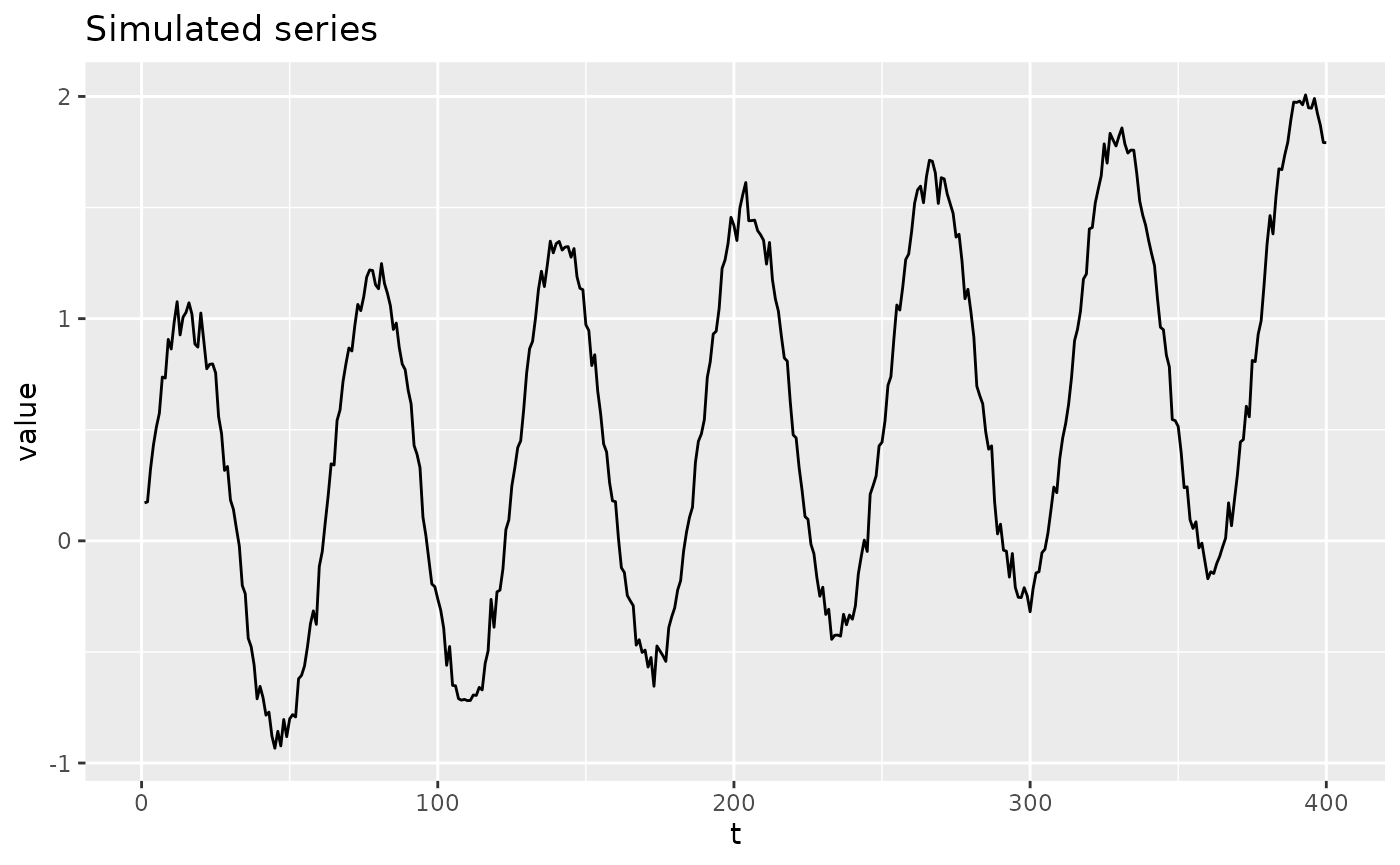

Because forecasting is temporally ordered, the train/test split must respect time: rsample::initial_time_split() takes the first proportion of rows for training and the remainder for testing, rather than a random shuffle.

split <- rsample::initial_time_split(series, prop = 0.8)
train_data <- rsample::training(split)
test_data <- rsample::testing(split)

Step 2: Build the Recipe

step_naomit() defaults to skip = TRUE, so the rows it drops (those without a complete future window) are only dropped when training; at predict time, future values are legitimately unknown, and the row is kept.

Both the window (predictor) and the lead columns (outcome) are derived from value by the recipe steps themselves, rather than existing as separate raw columns, so the recipe is built with recipe(train_data) (no formula) and each step assigns the role of the column(s) it creates (step_lead() defaults to role = "outcome", step_sequence() to role = "predictor").

rec <- recipe(train_data) |>
  step_lead(value, lead = seq_len(horizon), prefix = "lead_") |>
  step_naomit(starts_with("lead_")) |>
  step_sequence(value, timesteps = timesteps, new_col = "window")

Step 3: Define Layer Blocks and the Model Specification

The input block declares the (timesteps, features) shape, an LSTM layer summarizes the window, and a single output dense block emits all horizon forecasted values at once.

input_block <- function(input_shape) {
  layer_input(shape = input_shape, name = "window_input")
}
lstm_block <- function(tensor, units = 32) {
  tensor |> layer_lstm(units = units)
}
# `units` needs a default to work around a doc-generator quirk when handling
# args with no default; it is always overridden via `output_units` below.
output_block <- function(tensor, units = 1) {
  tensor |> layer_dense(units = units)
}

model_name <- "multistep_lstm_spec"
on.exit(remove_keras_spec(model_name), add = TRUE)

create_keras_functional_spec(
  model_name = model_name,
  layer_blocks = list(
    window = input_block,
    lstm = inp_spec(lstm_block, "window"),
    output = inp_spec(output_block, "lstm")
  ),
  mode = "regression"
)

Step 4: Fit and Forecast

output_units is set to horizon so the single output head predicts the full vector of future steps in one pass.

spec <- multistep_lstm_spec(
  lstm_units = 32,
  output_units = horizon,
  fit_epochs = 30,
  fit_verbose = 0
) |>
  set_engine("keras")

wf <- workflow(rec, spec)
fit_obj <- fit(wf, data = train_data)
#> 10/10 - 0s - 36ms/step

predict() returns a nested .pred list-column: one row per input sample, each holding a small tibble of .step (1 to horizon) and .pred (the forecasted value at that step). This mirrors how the censored package nests multiple survival-probability values per row (.pred / .eval_time / .pred_survival), nesting over forecast step instead of evaluation time.

preds <- predict(fit_obj, new_data = test_data)
#> 2/2 - 0s - 94ms/step
preds
#> # A tibble: 57 × 1
#>    .pred           
#>    <list>          
#>  1 <tibble [6 × 2]>
#>  2 <tibble [6 × 2]>
#>  3 <tibble [6 × 2]>
#>  4 <tibble [6 × 2]>
#>  5 <tibble [6 × 2]>
#>  6 <tibble [6 × 2]>
#>  7 <tibble [6 × 2]>
#>  8 <tibble [6 × 2]>
#>  9 <tibble [6 × 2]>
#> 10 <tibble [6 × 2]>
#> # ℹ 47 more rows

preds$.pred[[1]]
#> # A tibble: 6 × 2
#>   .step .pred
#>   <int> <dbl>
#> 1     1 0.826
#> 2     2 0.745
#> 3     3 0.624
#> 4     4 0.517
#> 5     5 0.404
#> 6     6 0.284

Step 5: Visualize the Forecast

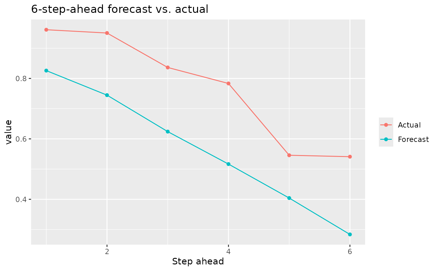
Unnesting .pred turns the forecast horizon for one starting point into a plain tibble, easy to compare against the actual future values.

one_forecast <- preds |>
  dplyr::slice(1) |>
  tidyr::unnest(.pred)

actual_future <- test_data$value[seq_len(horizon) + timesteps - 1]

comparison <- one_forecast |>
  dplyr::mutate(actual = actual_future)

ggplot(comparison, aes(.step)) +
  geom_line(aes(y = .pred, color = "Forecast")) +
  geom_point(aes(y = .pred, color = "Forecast")) +
  geom_line(aes(y = actual, color = "Actual")) +
  geom_point(aes(y = actual, color = "Actual")) +
  labs(
    title = "6-step-ahead forecast vs. actual",
    x = "Step ahead",
    y = "value",
    color = NULL
  )

Step 6: Uncertainty Intervals

type = "conf_int" and type = "pred_int" also work for this vector-valued output. Each forecast step gets its own last-layer Laplace posterior (its own prior precision and observation noise), sharing the same penultimate feature representation. This is the same independent-per-output treatment kerasnip already uses for separately named multi-output heads, generalized from “multiple Dense layers” to “multiple units of one Dense layer”. It lets uncertainty differ (and typically grow) across the horizon instead of a single pooled width applied to every step alike.

preds_ci <- predict(fit_obj, new_data = test_data, type = "conf_int")
#> 2/2 - 0s - 12ms/step
#> 2/2 - 0s - 12ms/step
#> 2/2 - 0s - 12ms/step
#> 2/2 - 0s - 12ms/step
#> 2/2 - 0s - 12ms/step
#> 2/2 - 0s - 12ms/step

comparison_ci <- preds_ci |>
  dplyr::slice(1) |>
  tidyr::unnest(.pred) |>
  dplyr::mutate(actual = actual_future)

ggplot(comparison_ci, aes(.step)) +
  geom_ribbon(aes(ymin = .pred_lower, ymax = .pred_upper), alpha = 0.2) +
  geom_line(aes(y = .pred, color = "Forecast")) +
  geom_point(aes(y = .pred, color = "Forecast")) +
  geom_line(aes(y = actual, color = "Actual")) +
  geom_point(aes(y = actual, color = "Actual")) +
  labs(
    title = "6-step-ahead forecast with 95% confidence intervals",
    x = "Step ahead",
    y = "value",
    color = NULL
  )

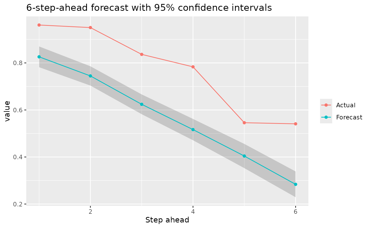
These are marginal per-step intervals: each step’s uncertainty is computed on its own, without modeling how errors at different steps co-move (e.g. an under-forecast at step 3 tending to also mean an under-forecast at step 4).

Step 7: Joint (Correlated) Prediction Intervals

predict(..., type = "pred_int", joint = TRUE) captures that co-movement. Instead of a single symmetric band per step, each forecast step’s own epistemic (weight) uncertainty is combined with a noise term that is sampled jointly across steps, using the empirical covariance of training residuals across the forecast horizon (the classic “seemingly unrelated regression” treatment of several linear outputs sharing one design matrix). 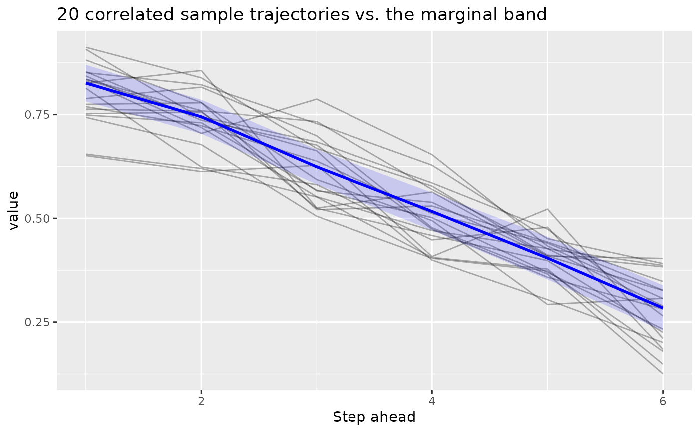The result is a set of correlated, internally-consistent sample trajectories rather than independent per-step guesses.

Rather than pre-summarizing these into another .pred_lower/.pred_upper band, the result is returned as raw draws tagged with a .draw column, the same convention tidybayes and the wider tidyverse Bayesian ecosystem use for “several posterior/predictive samples per observation”, so you can compute whatever joint or marginal summary you need with standard dplyr/tidyr tools.

preds_joint <- predict(
  fit_obj,
  new_data = test_data,
  type = "pred_int",
  joint = TRUE,
  n_draws = 200
)
#> 2/2 - 0s - 12ms/step

one_row_draws <- preds_joint$.pred[[1]]
one_row_draws
#> # A tibble: 1,200 × 3
#>    .draw .step .pred
#>    <int> <int> <dbl>
#>  1     1     1 0.835
#>  2     2     1 0.769
#>  3     3     1 0.851
#>  4     4     1 0.835
#>  5     5     1 0.743
#>  6     6     1 0.912
#>  7     7     1 0.655
#>  8     8     1 0.749
#>  9     9     1 0.813
#> 10    10     1 0.763
#> # ℹ 1,190 more rows

# Draws at different steps are correlated, unlike the marginal intervals above.
one_row_draws |>
  tidyr::pivot_wider(names_from = .step, values_from = .pred, names_prefix = "step_") |>
  dplyr::select(step_1, step_2) |>
  cor()
#>           step_1    step_2
#> step_1 1.0000000 0.3758853
#> step_2 0.3758853 1.0000000

A handful of individual sampled trajectories, plotted alongside the marginal band from Step 6, shows what the correlation buys you: real trajectories tend to stay consistently above or below the mean forecast across steps, rather than jittering independently step to step the way the marginal band alone would suggest.

sample_paths <- one_row_draws |>
  dplyr::filter(.draw <= 20)

ggplot(sample_paths, aes(.step, .pred, group = .draw)) +
  geom_line(alpha = 0.3) +
  geom_ribbon(
    data = comparison_ci,
    aes(x = .step, y = .pred, ymin = .pred_lower, ymax = .pred_upper),
    inherit.aes = FALSE,
    alpha = 0.15,
    fill = "blue"
  ) +
  geom_line(
    data = comparison_ci,
    aes(x = .step, y = .pred),
    inherit.aes = FALSE,
    color = "blue",
    linewidth = 1
  ) +
  labs(
    title = "20 correlated sample trajectories vs. the marginal band",
    x = "Step ahead",
    y = "value"
  )

Epistemic (weight) uncertainty is still treated independently per step even here; only the aleatoric noise term carries cross-step correlation. A fully joint treatment of epistemic uncertainty too would need a joint (Kronecker-factored) posterior over the entire last-layer weight matrix, which is not implemented. joint = TRUE is only available for type = "pred_int"; type = "conf_int" reflects epistemic uncertainty only, which this implementation has no estimated cross-step correlation source for.

Limitations

This is a v1 building block, not a full forecasting framework. In particular:

One ordered series at a time. step_sequence() windows the incoming data as a single series; grouped/panel forecasting (many independent series, e.g. per-store or per-sensor) is not handled automatically and would need windowing done per group before this recipe.
Fixed window and horizon. timesteps and horizon (via output_units) are set once per spec, not tuned automatically across varying window lengths.
Epistemic uncertainty is always per-step. joint = TRUE (Step 7) correlates the aleatoric noise across steps, but each step’s own model-weight uncertainty is still computed independently.

Conclusion

step_sequence() and step_lead() let a standard tidymodels recipe produce the (samples, timesteps, features) input and (samples, horizon) target shapes a recurrent kerasnip model needs, so a multi-step forecaster fits into the same recipe() |> workflow() |> fit() |> predict() flow as any other model in this package.